Varun Dey
How an LLM sees text: tokens and vectors
This is part 1 of a series on how AI chat agents like ChatGPT, Claude and Gemini actually work, written by a backend engineer for backend engineers. No ML background assumed. This part covers how text turns into numbers: tokens and vectors. Later parts cover what the model does with those numbers.
If you spend your days thinking about services, queues, caches and failure modes, the way LLMs are usually explained can feel like it was written for a different profession. “Neural networks”, “gradient descent” and “emergent abilities” don’t map onto anything in your mental toolbox.
So let’s skip that and start from the interface, the same way you’d approach any unfamiliar system.
The whole thing, as an API
An LLM is, at its core, one function:
def next_token_probabilities(tokens: list[int]) -> dict[int, float]:
    ...
It takes a list of integers (tokens) and returns a probability for every token in its vocabulary being the next one. That’s the entire interface. There is no separate “answer a question” endpoint; answering is something we build out of this one primitive, as later parts of the series show. (If this sounds like autocomplete, it is: the interface is identical. Why an interface that simple is enough to answer questions is the subject of part 3.)
Here is what a single call looks like. To keep it readable I’ll show tokens as words, though the model sees integers:
input:   "The cat sat on the"
output:  " mat" 41%   " sofa" 23%   " floor" 12%   " roof" 8%   ...   (one entry per token in the vocabulary)
One call gives you one next token and nothing more. To get a whole reply, you pick a token from that distribution, append it to the input, and call the function again. Repeat until the model signals it is done:
call 1:  "The cat sat on the"            -> picks " mat"
call 2:  "The cat sat on the mat"        -> picks "."
call 3:  "The cat sat on the mat."       -> picks <|end|>   (stop)

reply:   " mat."
As code, that loop looks like this:
def generate(prompt_tokens, max_new_tokens):
    tokens = list(prompt_tokens)                       # start with the prompt
    for _ in range(max_new_tokens):                    # hard cap on reply length
        probs = next_token_probabilities(tokens)       # the model call: one forward pass
        next_token = sample(probs)                     # choose one token from the distribution
        if next_token == END_OF_TEXT:                  # a special token meaning "I'm done"
            break
        tokens.append(next_token)                      # feed the choice back in as input
    return tokens[len(prompt_tokens):]                 # everything after the prompt is the reply
Two names in there are not defined in this part:
samplepicks a token from the probabilities. The simplest version takes the most likely one; real systems add controlled randomness. See part 2.END_OF_TEXTis a special token that the model itself predicts when a reply is finished. We’ll see how that works in part 3.
This is called autoregressive generation: each output token is fed back in as input for the next step. Every property of an LLM service that you’ll later care about (latency, streaming, cost, batching) follows from this loop.
Everything in this part is about the input to that function: how text becomes a list of integers, and how each integer becomes numbers that a neural network can work with.
Step 1: text becomes integers
The model never sees characters. A tokenizer splits text into chunks from a fixed vocabulary (typically tens of thousands to a couple hundred thousand entries) and maps each chunk to an integer ID.
"Backend engineers love idempotency"
  -> ["Back", "end", " engineers", " love", " id", "emp", "otency"]
  -> [10373, 408, 24983, 3021, 877, 2931, 38251]   (illustrative IDs)
Common words are one token. Rare words, code, and non-English text split into more pieces. A rough rule of thumb for English is that a token is about three-quarters of a word.
Why care? Because tokens are the unit of everything: pricing, rate limits, context size, and latency. A token is to an LLM service what a row is to a database or a request is to an API gateway.
Step 2: integers become vectors
A token ID is just a label, like a user_id. ID 5000 is not “close to” ID 5001 in any useful sense, and arithmetic on IDs means nothing. A neural network can only do arithmetic, so we need to convert each ID into numbers in which closeness carries meaning.
A warm-up: colors are vectors
You already know a system that does exactly this: RGB. A color is described by three numbers, saying how much Red, Green and Blue it contains.
              R     G     B
red         [230,   30,   30]
crimson     [220,   20,   60]
blue        [ 30,   30,  230]
Each column measures how much of one “ingredient” the color has. Going from a name to its numbers is a table lookup: the name crimson maps to [220, 20, 60]. Three things follow from this:
- Close numbers mean close colors. Red and crimson have similar numbers in every column. Blue looks nothing like either, and its numbers don’t either.
- Closeness can be a single number. Cosine similarity measures how closely two lists of numbers point in the same direction: 1 means the same direction, and values near 0 mean unrelated. Red vs. crimson scores about 0.99, and red vs. blue about 0.27.
- You can do math on them. Average red and blue and you get
[130, 30, 130], a purple. Blending vectors gives you something in between. We’ll use that idea in part 2.
Words work the same way, with thousands of columns
An embedding gives every token its own list of numbers, the way every color has its [R, G, B]. The numbers in such a list are called a vector. The differences between colors and tokens are the scale and where the columns come from:
| Colors (RGB) | LLM embeddings | |
|---|---|---|
| What is described | Colors | Tokens |
| Number of columns | 3 | Thousands (4,096 in many mid-size models) |
| Who picked the columns | Humans: red, green, blue | Training. They have no human-readable names |
| “Close” means | Looks similar | Is used in similar ways, so means something similar |
That third row is the important one. Nobody designs the columns of an embedding. The numbers start out random and are adjusted during training. The training signal is “predict the next token better”, so tokens that appear in similar contexts and lead to similar continuations get nudged toward similar numbers. You can’t point at column 1,207 and say “this measures animal-ness”. The meaning lives in the overall pattern across all the columns. But the geometry works just as it does for colors: after training, “cat” and “dog” have similar numbers (like red and crimson), and “Paris” is far away from both.
You can watch this happen. The animation below is a real training run of a tiny model on 18 short sentences (about animals and about capital cities), with just 2 columns per word so that we can draw each word as a dot. Every dot starts at a random position. As training proceeds, each word’s numbers get adjusted so that the word predicts its neighbours a bit better, and the dots drift:
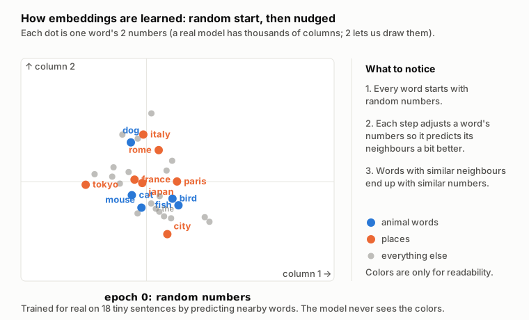
Nobody told the model that “cat” and “dog” are animals. They ended up together because they appear in similar sentences. Notice that the countries (italy, france, japan) formed their own group, apart from the cities: in the training text they show up in different contexts (“the capital of italy” versus “i visited paris”). The colors are only there for readability; the model never sees them.
The code behind this animation is on GitHub, and it runs with nothing but Python. Try changing the training sentences, for example by adding “i saw a fish in rome” and “a bird was eating fish in tokyo”, and re-run it to see how the picture changes. The README walks through what happens.
Here is a toy version with 4 columns instead of 4,096. Pretend the columns mean something like “animal”, “pet”, “place” and “city”. In a real model they don’t have such labels, but the geometry is the same:
         animal     pet   place     city
cat    [    0.9,    0.8,    0.1,     0.0 ]
dog    [    0.8,    0.9,    0.2,     0.1 ]
Paris  [    0.0,    0.1,    0.9,     0.8 ]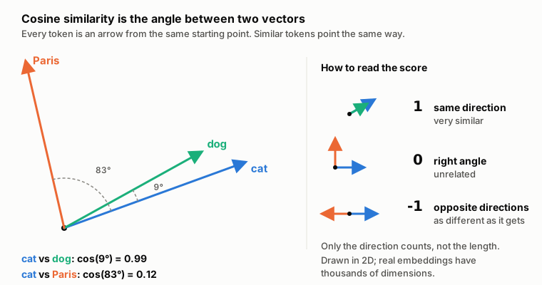
Picture each vector as an arrow from a shared starting point. Cosine similarity is the cosine of the angle between two arrows, which boils down to “how closely do they point the same way?”. cat and dog point almost the same way (about 9° apart) and score 0.99. cat and Paris are about 83° apart, close to a right angle, and score 0.12.
Only the direction matters, not the length. Dark red [139, 0, 0] and bright red [255, 0, 0] score exactly 1, because they point the same way. (The picture is drawn in 2D, but the idea is identical with 4,096 columns.)
The formula, if you want it
import math

def cosine_similarity(a, b):
    dot = sum(x * y for x, y in zip(a, b))              # multiply column by column and add up
    length_a = math.sqrt(sum(x * x for x in a))
    length_b = math.sqrt(sum(x * x for x in b))
    return dot / (length_a * length_b)                  # divide the lengths out, so only direction is left

cosine_similarity([230, 30, 30], [220, 20, 60])         # red vs crimson -> 0.99
cosine_similarity([230, 30, 30], [30, 30, 230])         # red vs blue    -> 0.27
If you’ve worked with vector search, this is the same idea: vector databases use vectors like these to find similar text (we’ll get to them in the retrieval part of the series). Those come from dedicated embedding models rather than from the lookup table inside an LLM, but the geometry works the same way.
The embedding table
Inside the model, the lookup is a big table with one row per vocabulary entry, and looking up a token is a plain array index:
embedding_table = load_weights("embeddings")    # shape: [vocab_size, d_model], e.g. [100_000, 4096]

vector = embedding_table[token_id]              # one row: a list of 4096 floats
# [0.012, -0.83, 0.27, ... ]
Think of it as a database table with a fixed schema:
- Rows: one per token in the vocabulary. With a 100,000-token vocabulary, that’s 100,000 rows.
- Columns: a fixed number of floats per row. That number is called
d_model(the “model dimension”, or width), and it plays the role of the 3 in RGB. It’s chosen by the model’s designers: many mid-size open models use 4,096, and bigger models use more. Every vector inside the model has exactly this length, from the first lookup to the last layer, much like every record in a table has the same columns.
So each token is represented by 4,096 numbers, and the whole table holds 100,000 × 4,096 ≈ 410 million numbers.
How much memory is that? Models usually store each number in 16 bits (2 bytes), so the table takes 410 million × 2 bytes ≈ 0.8 GB. That’s a lot for what is just a lookup table, and it’s only one component of the model. This table is part of the weights: the learned numbers saved alongside the model, loaded into GPU memory when a server starts up, and read-only afterwards. We’ll look at the full memory picture in part 2.
Order matters too
A plain table lookup treats the prompt as a bag of tokens, and “dog bites man” would look the same as “man bites dog”. So the model also injects each token’s position into its vector, either by adding a position-dependent signal or, in most modern models, by encoding position inside the attention step (part 2). You don’t need the details; just know that the vectors entering the first layer carry both “which token” and “where”.
A whole prompt is a grid
So far we’ve looked up one token. But a prompt has many tokens, and the model processes all of them together. Here is what that looks like for the three-token prompt “The cat sat”. To keep the numbers readable, pretend d_model is 4 instead of 4,096.
Step one: look up each token’s vector, exactly as above.
vec_the = embedding_table[id_of("The")]      # [ 0.1, -0.3,  0.7,  0.2 ]
vec_cat = embedding_table[id_of(" cat")]     # [ 0.9,  0.8,  0.1,  0.0 ]
vec_sat = embedding_table[id_of(" sat")]     # [-0.4,  0.5,  0.3,  0.9 ]
Step two: stack them in prompt order, one per row. The result is a matrix, which just means a 2D grid of numbers (a 2D array):
                    col 1   col 2   col 3   col 4
row 1  "The"      [  0.1    -0.3     0.7     0.2 ]
row 2  " cat"     [  0.9     0.8     0.1     0.0 ]
row 3 " sat" [ -0.4 0.5 0.3 0.9 ]- Each row is one token’s vector, and the rows are in the same order as the tokens in the prompt, so row 2 always means “the second token”.
- The number of columns is
d_model(the “width”). In a real model that’s 4,096 columns instead of 4. - The number of rows is N, the number of tokens in the prompt. A 3-token prompt gives 3 rows, and a 10,000-token prompt gives 10,000 rows.
So the grid for “The cat sat” in a real model has 3 rows and 4,096 columns. People write this as its shape: [3, 4096], or [N, d_model] in general.
A shape is a count, not a last index. Indexing starts at 0, so the columns are numbered 0 to 4095, but there are still 4,096 of them, exactly like len([0] * 4096) is 4096 even though the last valid index is 4095. Likewise, the 3 rows are numbered 0 to 2, and the shape says 3.
That grid is what goes into the model’s layers. What the layers do with it is the subject of part 2.
What’s next in the series
- How an LLM sees text: tokens and vectors (this post)
- How an LLM understands context: layers and attention. How each token’s vector gets enriched with context, and how the model picks the next token.
- Anatomy of a chat request. Chat templates, statelessness, context windows and prompt caching.
- LLM inference: serving is a scheduling problem. KV cache, continuous batching, and why GPU memory is the scarce resource.
- Retrieval, tools and agents. Why an agent is a distributed workflow with a flaky, non-deterministic step.
- Training at scale. Distributed training as a fault-tolerance problem.
In part 2 we’ll open up the model and see what happens to this grid of vectors.